Making the Most out of the Money Cards
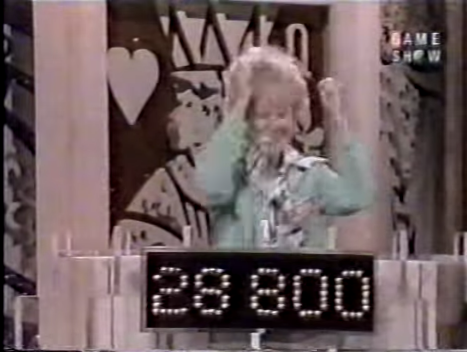
The game itself was based on the old gambling card game of Acey-Deucey. As such, it is ripe for strategic and mathematical evaluation. While we will no doubt one day look at the proper strategy in the front game, today we’re going to take a closer look at the “Money Cards” bonus round. This was one of the most exciting and lucrative bonus rounds around in the 1970’s, where a contestant, if armed with enough skill and backbone, could parlay $200 into $28,800. But how should one play the Money Cards to maximize one’s winnings? Should a player even play to maximize their winnings?
The Rules
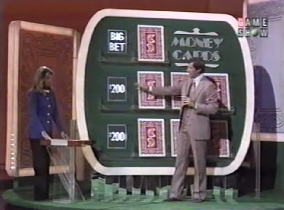
After the fourth card is turned over, play proceeds to the second row and the contestant is given another $200. Contestants keep wagering, following the same rules up until the last higher/lower decision on the top row, where the minimum bet becomes half of the player’s total. In addition, the player may choose to swap the face-up card before the first, fourth, and seventh decision (the first card on each level) with a new card from the deck.
While some of the rules changed during the run of the show (the ramifications of which we will address later), this set of rules will be the basis of our discussions.
Strategy
Some of the simpler aspects of the game are easy to analyze. We know that in a deck of cards, the “8” card is the midpoint – there are 24 cards lower and 24 cards higher than it. We should thusly wager on the next card being higher when our base card is lower than 8, and lower when the base card is higher than an 8. When the card is an 8, we can count the cards we’ve seen (not a difficult task in the end game, as almost all cards remain visible when after they are played), and determine whether there are more higher and lower cards in the deck, and predict using this knowledge.
When it comes to choosing whether or not to switch our base card when given the opportunity, we can analyze our chance of success with every base card, as seen in the following table:
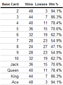
Using this data, we can determine that we have on average, a 72.4% chance of calling the next card correctly given a random base card. Therefore, it makes sense to switch our base card when our chances of winning are below that number. Using the table above, we see that we should switch on any card between a 5 and Jack.
Betting Strategy – The Naive Approach
It’s clear that we should bet the minimum when we are faced with an 8 that we can’t change – barring a large number of lower or higher cards already used, it’s going to be a net loser, so we should minimize our losses. But what about the other 12 cards?
For our purposes, let’s define a betting strategy as a series of 6 percentages, representing the percentage of your bank that you should bet depending upon your face up card. Why only 6 instead of 12? Because the chances of winning with a 2 are the same as winning with an Ace, the chances of winning with a 3 are the same as a King, and so forth. We only need 6 percentages to cover all twelve possibilities.
For example, the following would be a betting strategy: 30%|50%|70%|80%|90%|100%. These represent the percentage of your bank that you will bet, depending on the face-up card. If you are facing a 7 or a 9, you bet 30% of your bank, the left-most percentage. If you are blessed with an Ace or a 2, you bet the right-most percentage. If a betting strategy’s wager falls below the minimum bet allowed, then you would instead bet the minimum.
Let’s envision a theoretical contestant, All-In Adrian. He’s a smart gambler, so he knows that when you’re offered even money on a better than even money proposition, you should bet heavily. In this case, he’s going to bet everything on every card, as long as it’s not an 8. His betting strategy would be 100%|100%|100%|100%|100%|100%.
Adrian is correct, you should bet heavily when the odds are in your favor. He’s found the strategy that will earn him the most money on average. But is that the necessarily the best strategy?
Betting Strategy – The Nuanced Approach
Let’s look at another theoretical contestant, Nervous Nick. Nick hates gambling and hates to lose. He’s going to do nothing but wager the minimum bet of $50 every time except for the last, where he’ll bet the new minimum of half of whatever he has left. His strategy would be written as 0%|0%|0%|0%|0%|0%.
Something funny happens when you compare Nick and Adrian’s strategies. On average, Adrian is going to win a heck of a lot more money than Nick. But if you were to look at who would be more likely to have more money after each contestant played one round, Nick would be ahead most of the time.
This speaks to the risk involved in Adrian’s strategy. Sure, in the long run, he would come out ahead. But in the meantime, he’s going to go bust about 70% of the time, while Nick is guaranteed to walk away from the game with some money. And, unfortunately for Adrian, there is no long run. Most contestants would only get the privilege of playing the Money Cards once or twice before losing the front game and having to leave the show. Adrian’s strategy would be great if he could play the game unlimited times, but that’s just not the case.
Risk
What we want to do is analyze every possible betting strategy. We’ll look at the expected value of the strategy, and to represent the risk we’ll use the standard deviation that the strategy creates. The higher the standard deviation, the more volatile the possible range of values, and the higher the risk. However, analyzing every possible combination of six percentages would be extremely overwhelming. We’ll limit the amount of possible strategies by doing two things:
- Every percentage must be less than or equal to the next percentage in line. This makes sense – there’s no reason why you would ever, say, wager 40% on a 6 but only 30% on a 5.
- We’ll limit our percentages to increments of 10%. We’re already losing precision in our potential betting strategies by being forced to wager in $50 increments, so the precision we lose by limiting ourselves to 10 percent increments is not that much.
Those two rules took our potential number of strategies down to a manageable 8,008. We then ran a Monte Carlo simulator to determine the expected value and standard deviation of each strategy. When looking at the results, we found that we could eliminate a large number of potential strategies from consideration. To see why, we plotted each strategy’s expected value and standard deviation onto a scatter chart:
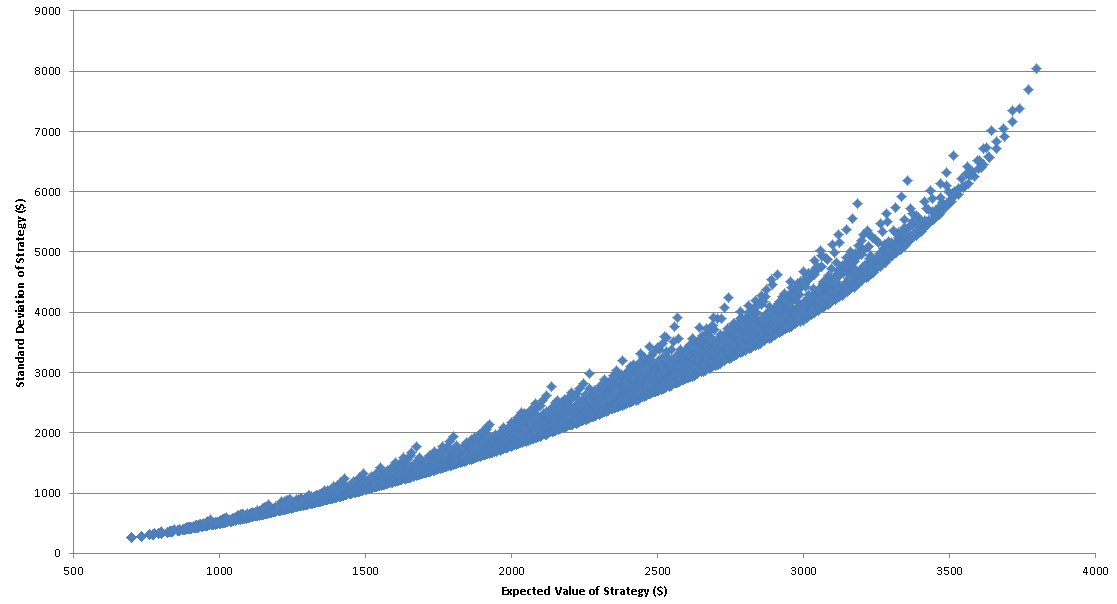
The general shape of the graph forms a curve sloping upwards. In modern portfolio theory, the points on the curve form what is known as the efficient frontier. The points that form this curve are the strategies that offer the highest value for a given level of risk. Strategies that do not form part of this curve are not optimal, as they offer less return for their risk than another strategy would.
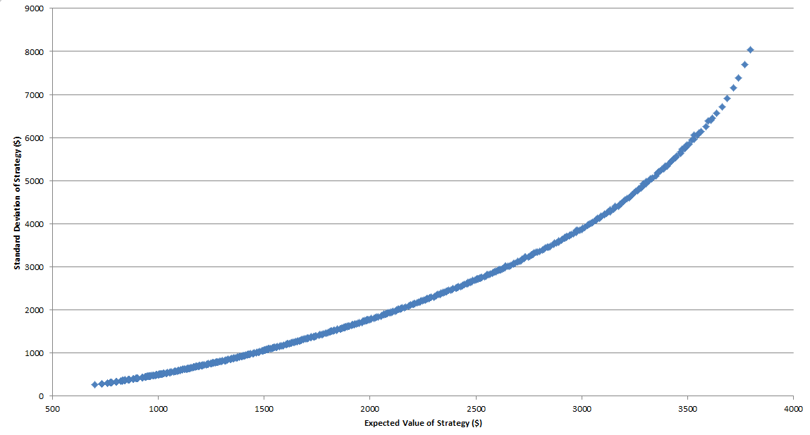
Let’s take a look at an individual example involving two potential strategies: Strategy A (40%|40%|40%|50%|50%|90%) and Strategy B (0%|0%|30%|50%|60%|100%) Strategy A was determined to have a value of $1,768.28 with a deviation of $1,562.92. Strategy B has a value of $1.807.79 and a deviation of $1,496.47. Since Strategy B has both a higher value and lower risk than the Strategy A, there’s never a reason to use Strategy A. Thus, we can discard Strategy A from further analysis.
Removing these inefficient strategies leaves us with a group of 647 viable strategies. Updating our scatter point chart shows us the efficient frontier in clearer detail.
Unfortunately, this is where our search for an “optimal strategy” has to end. Each of these 647 strategies is as viable as the next from a mathematical viewpoint. It only depends on how much risk you wish to undertake in the pursuit of profit.
Personal Strategies
Luckily, we can use the standard deviation of a distribution to determine how likely a given event is to occur. Given a dollar value, we can find how many standard deviations away from the mean each strategy is, and find the strategy that will give you the highest chance of achieving that dollar value by finding the strategy the lowest number of standard deviations away from the mean.
For example, say you wanted to find the strategy that gave the you highest chance of winning at least the modest sum of $500. Then you’d want to use the strategy 0%|0%|0%|20%|30%|50%, where $500 is -1.012 standard deviations away from the mean, corresponding to an estimated chance of 84.4% of making at least $500. If you wanted to shoot higher and maximize your chances of making $2,500, then the riskier strategy of 50%|90%|100%|100%|100%|100% would give you the best chance.
Rule Changes
The Money Cards underwent several rule changes over the years, each in the favor of the contestants. Two years into the show’s run, the rule concerning ties changed. Where before ties were considered losses (meaning it would be possible to lose on an Ace or 2), ties were now considered pushes – no money was gained or lost if the same card came up twice. For one thing, this now meant that all strategies should end in 100% for Aces and 2’s, since there was no possible way to lose money. It also would allow contestants to play more conservatively to find the best strategy for minimum values.
When the show was revived in 1986, two major rule changes happened to the Money Cards. Firstly, the amount of money given to the contestant upon reaching the second row was increased to $400, making the top prize a round $32,000. The second big change had to do with when the contestant could change cards. Now, instead of just the first card on each level being changed, you could change any card at any time, but only once per level. This complicated the strategy involving choosing when to change cards, the analysis of which we will leave for another time.
Our Final Answer
In case you want to try these strategies out yourself, we’ve created a series of charts which will give you the ideal strategy given the minimum amount you want to win for any of the three rule sets. While we can’t point to a single strategy and say it’s the best strategy to follow, looking at these charts and gauging how risky you would want to be would take you a long way to maximizing your potential earnings.