1000 Heartbeats: When to Cashout?
You know what they say about the Deputy Undersecretary of the Interior, they’re only 1,000 heartbeats away from the Presidency.
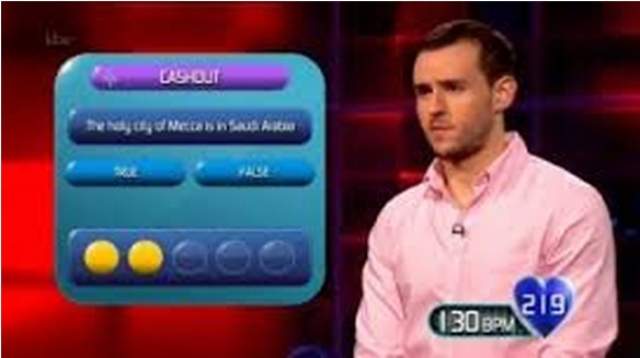
ITV debuted a new game show on February 23rd, 1000 Heartbeats. The main gimmick of the show is that the contestant’s own heartbeat determines how long they have to play. It’s a stylish show, complete with a live string quartet providing the music at the same tempo as the contestant’s heart rate, and has been getting favorable reviews.
The contestant is given a “clock” of 1000 of their own heartbeats (measured by a well-hidden heart monitor) to play a series of minigames testing the contestant’s skills in anagrams, mental arithmetic, and general knowledge. Each successfully completed minigame increases the potential winnings of the contestant, up to a maximum of £25,000. However, if they run out of heartbeats, their game is over and they leave empty-handed. After each game is completed, the contestant is given a preview of the next game and, taking into consideration the number of heartbeats they have remaining, may either play on for more money or stop. However, before the contestant can walk away with their money, they must play one final minigame with the remainder of their heartbeats, named Cashout.
My cardiologist’s new stress test has yet to be endorsed by the American Heart Association.
Cashout is a fairly simple game. As their heartbeats tick down, the contestant is given a series of True or False statements, and must correctly answer 5 in a row in order to win. Giving an incorrect answer not only forces them to start their chain of 5 answers over again, but also deducts 25 heartbeats from their clock. It’s an effective denouement, and has provided us with tense finishes already in the show’s short history. But watching it got me thinking – how many heartbeats would you want to bring into Cashout to maximize your chance of success? And when during the course of the game is it ideal to play Cashout instead of pressing onward for a potentially higher payday?

People were shocked to see the bold new direction being taken by Brian Eno.
Before we can measure how successful a contestant will be in Cashout, we first need to determine what metrics we can measure that will allow us to estimate a contestant’s success. I’ve identified three metrics: what their heart rate is, how often they give the correct answer, and how long each question takes to read and answer. Using those three variables, we can figure out the odds of completing a sequence of 5 correct answers, and how many heartbeats would elapse during that time.
These metrics will be different for each player, but for the purposes of this article, we will create an average contestant, using the data from the contestants who played during the first five episodes. In Cashout, the average contestant would answer 70.14% of the True/False questions correctly, while taking 6.45 seconds per question with a heart rate of 128 BPM. Using these values, we ran a Monte Carlo simulation to determine the chance that the average contestant will successfully complete Cashout given the number of heartbeats they started with. The results are displayed in this graph.
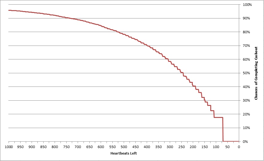
It’s a curve that starts declining fairly gently, but increases in slope before crashing to 0% around 70 heartbeats That’s the minimum number of heartbeats needed to see and answer 5 questions correctly with no wrong answers It may not have have happened during the first week of shows, but it should happen 17.5% of the time. Starting Cashout with anything above 250 heartbeats leads to a better than 50% chance of succeeding.
We can use these values to help decide whether or not to proceed to the next round during gameplay. At any given point in a player’s game, we can calculate the Expected Value (EV) of the game, which is the amount of money the player would win on average if they played Cashout. That value is determined by the amount of money banked so far multiplied by their chances of completing Cashout with their remaining heartbeats. For example, if a contestant has £500 banked, and has a 90% chance of winning Cashout with their remaining heartbeats, the EV of their game at that point would be £450.
If it’s a good idea for the contestant to play onward, the EV of their game after the next round must be higher. We can represent this in the following formula:
![]()
M is the amount of money currently banked, H is the number of Heartbeats remaining, and C is the function that tells us the chances of winning Cashout given a number of heartbeats, as defined by the chart above. M’ and H’ are the money and heartbeats left after the next round is played.
This function will be easier to work with if we divide both sides by M’, as so:
![]()
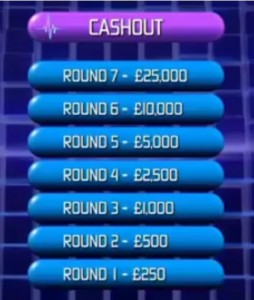 We now see that the contestant should want to move on if their future chances are greater than their current chances multiplied by the ratio at which the banked money will increase. Looking at the money ladder, we can see that in rounds 2, 3, 4, and 6 the money doubles, and M divided by M’ would be .5. Thus, the contestant should move on if their chances of winning Cashout are greater than half of their current chances. In rounds 3 and 7, the jump is greater, as the money is increased 150%. M divided by M’ in this case would be .4, so the contestant’s future chances can drop by as much as 60% of their current level before moving on becomes a bad idea.
So, we know the ratio at which our money rises, and we can determine our current chances of winning Cashout. But how can you determine your future chances? After all, you don’t know exactly how many heartbeats you’ll have left. This is the position in the game where an element of estimation comes into play. Taking a look at your past performances as well as the difficulty level of the next game, you’ll have to estimate how many heartbeats you’ll think you’ll need to successfully complete the next game.
Here’s that data broken down in graph form. The two lines represent the break-even points of how many heartbeats you can spend given your current number of heartbeats, depending on what round you are playing.
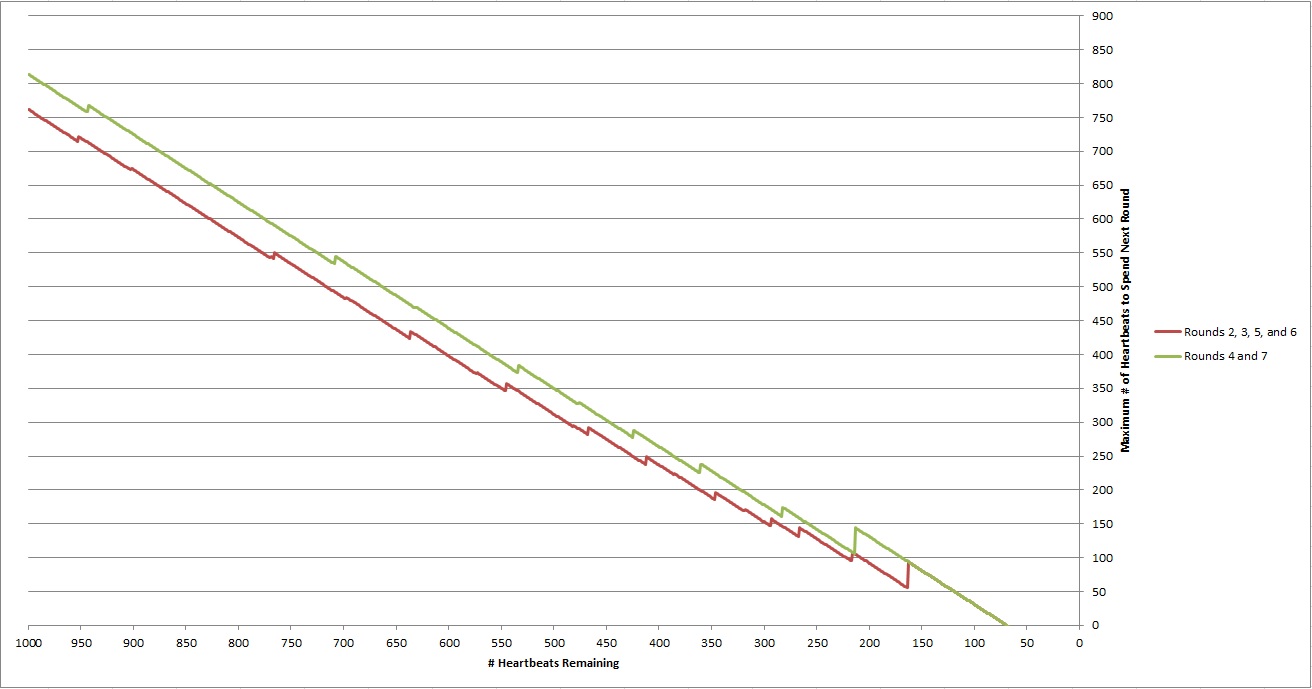
Click to see the full-size chart.
Let’s use this data to take a closer look at the two contestants who completed games on the show that aired on March 2nd.
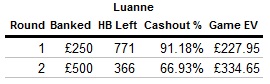
Luanne had a relatively poor first round of Contrast, and continued the theme with an even worse attempt at Unravel in round 2. By the time Round 3 came along, she only had 366 heartbeats left to play Assemble. According to the chart above, Luanne should have continued to play if she thought that she could complete Assemble in fewer than 200 heartbeats. Since she hadn’t done that yet in her game, it was probably a wise move that she opted to play an early Cashout. Taking 366 heartbeats into Cashout should be enough for an average contestant to win about two-thirds of the time. In this particular example, she managed to play Cashout successfully, ending with a scant 6 heartbeats remaining and taking home a hard-earned £500.
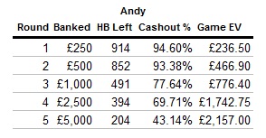
Andy blew threw Contrast and Unravel before hitting a stumbling block in round 3 with Assemble. He righted the ship in Round 4 with Link, and faced a decision on whether to play Keep Up, a mathematical game, in round 5. It seems like most players are loathe to play these games requiring mathematical computation, but Andy opted to continue playing. This could be seen as an aggressive move, but is a move that should lead to more money won as long as he spends fewer than 231 heartbeats on the game. He only spent 190, which increased the expected value of his game by £414.25. With only 204 heartbeats remaining, he had an easy choice to opt for Cashout at this point. Unfortunately, he quickly exhausted his heartbeats with a series of wrong answers, and wound up not converting his banked £5,000. Andy made a risky, yet mathematically sound choice to play Keep Up, but was not rewarded in the end.
Estimating how many heartbeats each minigame would take to complete would be very useful, We could could look at the past playings of each minigame and determine the time taken to complete it. However, after only five episodes, the data we would get would not be very reliable due to the small sample size. Perhaps if ITV gives this show the run it deserves, we will revisit this topic in a future article.
 The game of
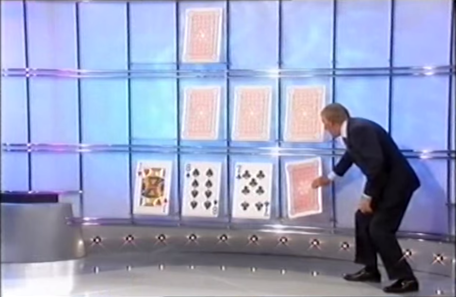
 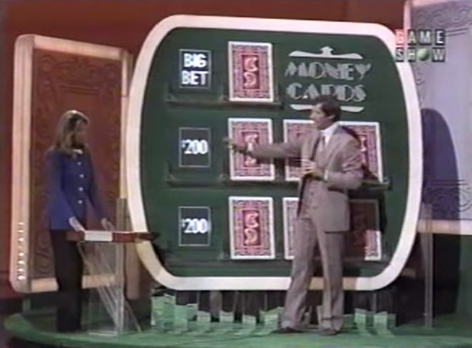 Seven cards are laid out on three rows, as seen in the image to the right. An eighth card is turned face up, and the contestant wagers any or all of their bank on whether the next card will be higher or lower (Aces are high). The contestant is staked $200 at the beginning of the round, and must bet in $50 increments, with a $50 minimum bet. Guessing correctly wins the amount bet, guessing incorrectly (even tying) results in the bet being lost.
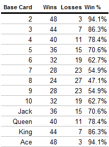
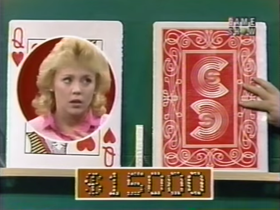 The story of Nick and Adrian shows that we can’t just look at the raw value of a strategy in our analysis; we have to consider risk as well. And that’s going to complicate matters. We can’t find a strategy that creates a mathematically proven equilibrium between value and risk – such a strategy doesn’t exist. As any economist or sociologist would tell you, different people quantify the risk/reward ratio differently. But, just because we can’t provide the solution, doesn’t mean we can’t provide a solution.
 Now, we could leave it here, and allow you to select a strategy based on your personal level of risk, but standard deviation doesn’t do a very good job of measuring risk aversion. If a person says “I’m willing to accept a standard deviation of $3,000”, what does that really mean? It’s clear we have to reframe the question if these results are going to be worth anything.